How To Make Excel Sheet Alternate Row Colors

How To Make Excel Sheet Alternate Row Colors. Select new table style. (image credit: Pick a table style that has alternate row shading.

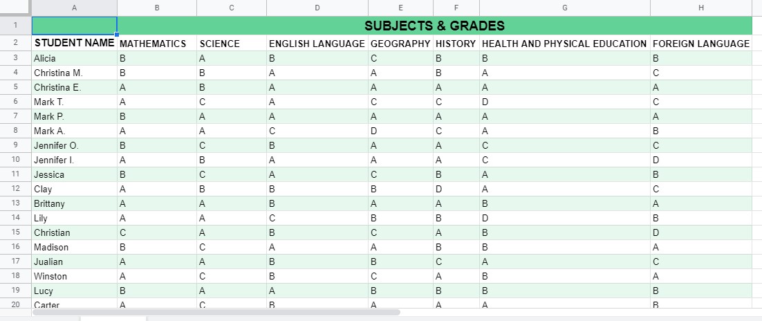
How to Color Alternate Rows in Google Sheets StepByStep Sheetaki from sheetaki.com

In the new formatting rule dialog box, click use a formula to determine cells to format under the select a rule type as former, and then enter this formula =iseven ($d2) ( d2 is the first cell of the. To apply the shading to the. To shade alternate rows in excel, use conditional formatting or apply a table style.

Source: wallseat.co

To color all alternating rows in the whole sheet, click the select all (triangle) button on the top left of the sheet. Go to the home tab > fill color (in the font group) and choose the color you want (you can also.

Source: candid.technology

To alternate row color in excel, you can do so by applying conditional formatting, with a combination of functions. Go to the home tab > fill color (in the font group) and choose the color you want (you can also.

Source: candid.technology

Applying alternate color and unique color to the data is to make the sheets more perfect which makes the data to view it in a colorful format. Select new table style. (image credit:

Source: usermanual.wiki

Applying alternate color and unique color to the data is to make the sheets more perfect which makes the data to view it in a colorful format. How to alternate row color in excel?

Source: www.ablebits.com

To shade alternate rows in excel, use conditional formatting or apply a table style. Pick a table style that has alternate row shading.

Source: usermanual.wiki

To change the shading from rows to columns, select the table,. How to alternate row color in excel with a formula select the range of cells you wish to edit.

Source: sheetaki.com

This rule uses a formula to determine whether a row is even or odd. Click home > format as table.

To Change The Shading From Rows To Columns,.

If you want the entire spreadsheet to have alternating rows, select the. Applying alternate color and unique color to the data is to make the sheets more perfect which makes the data to view it in a colorful format. Pick a table style that has alternate row shading.

Click Home > Format As Table.

Pick a table style that has alternate row shading. Select new table style. (image credit: To apply the shading to the.

As The Alternate Rows Are Not Adjacent Rows, We Have Selected Them By Pressing Ctrl.

Click home > format as table. Fill the first and second rows with the different colors you want. Select the range of cells that you want to format.

Select The Range Of Cells That You Want To Format.

This rule uses a formula to determine whether a row is even or odd. Select first row stripe and click ok. alternatively, you can alternate column colors utilizing this same method. In the new formatting rule dialog box, click use a formula to determine cells to format under the select a rule type as former, and then enter this formula =iseven ($d2) ( d2 is the first cell of the.

To Color All Alternating Rows In The Whole Sheet, Click The Select All (Triangle) Button On The Top Left Of The Sheet.

In microsoft excel, we can either apply color to. To alternate row color in excel, you can do so by applying conditional formatting, with a combination of functions. How to alternate row color in excel with a formula select the range of cells you wish to edit.